Basic API Reference
1. States and Gates
Here are a few examples of states and gates:
import numpy as np
from mrmustard.lab import *

vac = Vacuum(num_modes=2)        # 2-mode vacuum state
coh = Coherent(x=0.1, y=-0.4)    # coh state |alpha> with alpha = 0.1 - 0.4j
sq  = SqueezedVacuum(r=0.5)      # squeezed vacuum state
g   = Gaussian(num_modes=2)      # 2-mode Gaussian state with zero means
fock4 = Fock(4)                  # fock state |4>

D  = Dgate(x=1.0, y=-0.4)         # Displacement by 1.0 along x and -0.4 along y
S  = Sgate(r=0.5)                 # Squeezer with r=0.5

BS = BSgate(theta=np.pi/4)          # 50/50 beam splitter
S2 = S2gate(r=0.5)                  # two-mode squeezer
MZ = MZgate(phi_a=0.3, phi_b=0.1)   # Mach-Zehnder interferometer
I  = Interferometer(8)              # 8-mode interferometer
L  = Attenuator(0.5)                # pure lossy channel with 50% transmissivity
A  = Amplifier(gain=2.0, nbar=1.0)  # noisy amplifier with 200% gain
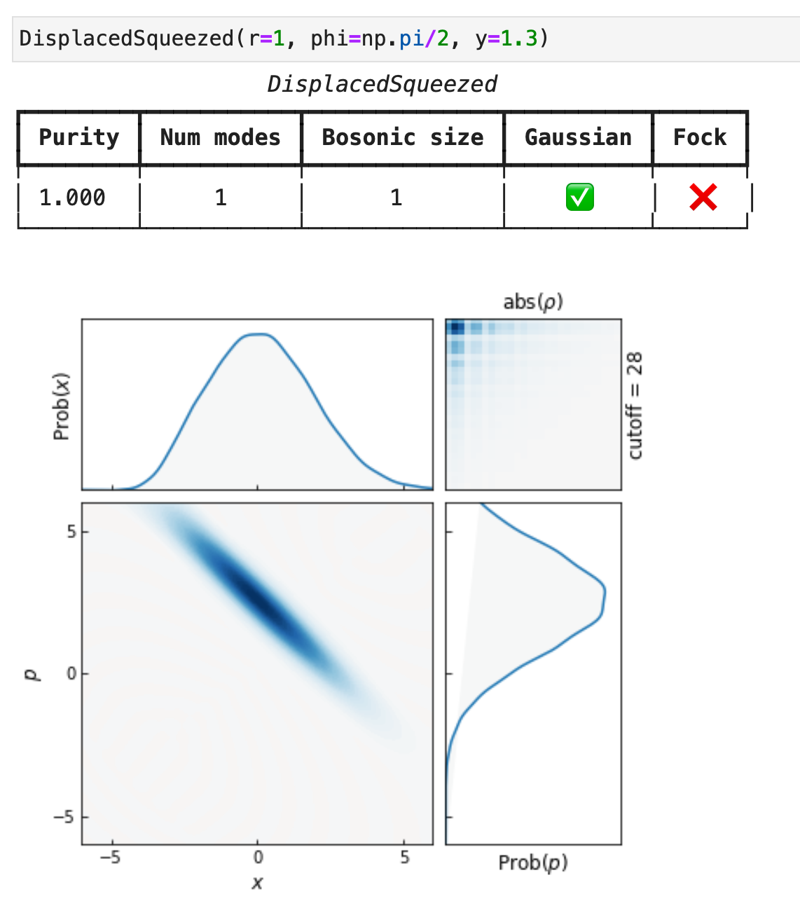
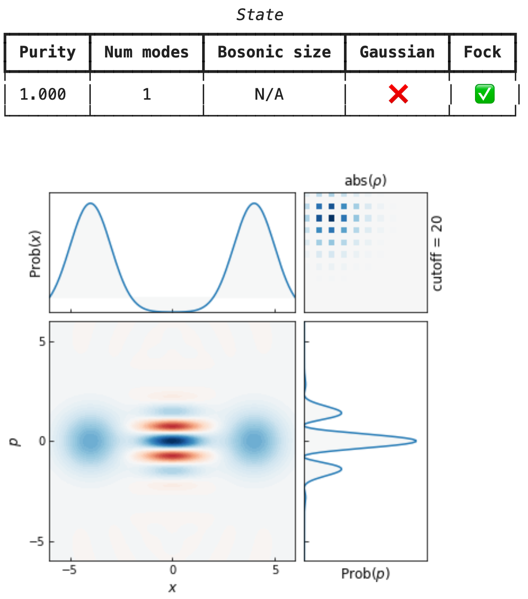
The repr of single-mode states shows the Wigner function:
cat_amps = Coherent(2.0).ket([20]) + Coherent(-2.0).ket([20])
cat_amps = cat_amps / np.linalg.norm(cat_amps)
cat = State(ket=cat_amps)
cat
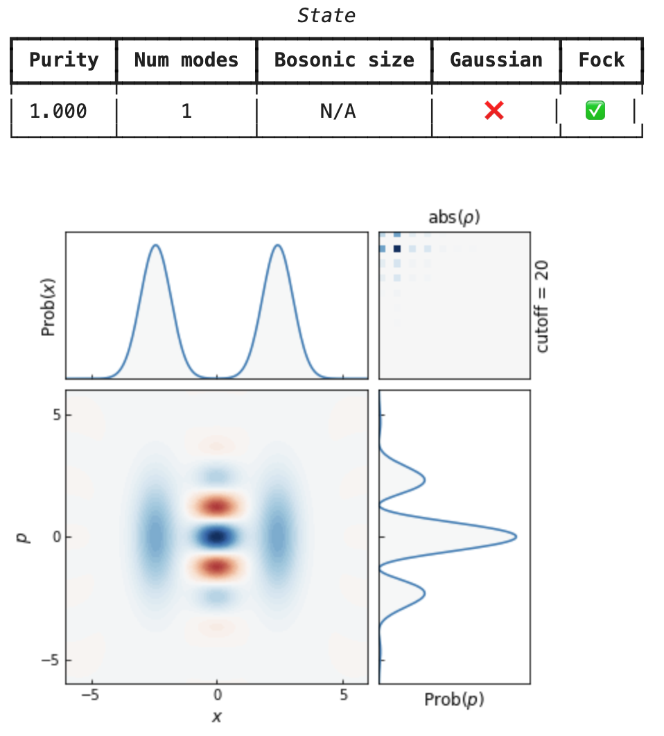
States (even those in Fock representation) are always compatible with gates:
cat >> Sgate(0.5) # squeezed cat
2. Gates and the right shift operator >>
Applying gates to states looks natural, thanks to python’s right-shift operator >>:
displaced_squeezed = Vacuum(1) >> Sgate(r=0.5) >> Dgate(x=1.0)
If you want to apply a gate to specific modes, use the getitem format. Here are a few examples:
D = Dgate(y=-0.4)
S = Sgate(r=0.1, phi=0.5)
state = Vacuum(2) >> D[1] >> S[0]  # displacement on mode 1 and squeezing on mode 0

BS = BSgate(theta=1.1)
state = Vacuum(3) >> BS[0,2]  # applying a beamsplitter to modes 0 and 2
state = Vacuum(4) >> S[0,1,2]  # applying the same Sgate in parallel to modes 0, 1 and 2 but not to mode 3
3. Circuit
When chaining just gates with the right-shift >> operator, we create a circuit:
X8 = Sgate(r=[1.0] * 4) >> Interferometer(4)
output = Vacuum(4) >> X8

# lossy X8
noise = lambda: np.random.uniform(size=4)
X8_realistic = (Sgate(r=0.9 + 0.1*noise(), phi=0.1*noise())
                >> Attenuator(0.89 + 0.01*noise())
                >> Interferometer(4)
                >> Attenuator(0.95 + 0.01*noise())
               )

# 2-mode Bloch Messiah decomposition
bloch_messiah = Sgate(r=[0.1,0.2]) >> BSgate(-0.1, 2.1) >> Dgate(x=[0.1, -0.4])
my_state = Vacuum(2) >> bloch_messiah
4. Measurements
In order to perform a measurement, we use the left-shift operator, e.g. coh << sq (think of the left-shift on a state as “closing” the circuit).
leftover = Vacuum(4) >> X8 << SqueezedVacuum(r=10.0, phi=np.pi)[2] # a homodyne measurement of p=0.0 on mode 2
Transformations can also be applied in the dual sense by using the left-shift operator <<:
Attenuator(0.5) << Coherent(0.1, 0.2) == Coherent(0.1, 0.2) >> Amplifier(2.0)
This has the advantage of modelling lossy detectors without applying the loss channel to the state going into the detector, which can be overall faster e.g. if the state is kept pure by doing so.
5. Detectors
There are two types of detectors in Mr Mustard. Fock detectors (PNRDetector and ThresholdDetector) and Gaussian detectors (Homodyne, Heterodyne). However, Gaussian detectors are a thin wrapper over just Gaussian states, as Gaussian states can be used as projectors (i.e. state << DisplacedSqueezed(...) is how Homodyne performs a measurement).
The PNR and Threshold detectors return an array of unnormalized measurement results, meaning that the elements of the array are the density matrices of the leftover systems, conditioned on the outcomes:
results = Gaussian(2) << PNRDetector(efficiency = 0.9, modes = [0])
results[0]  # unnormalized dm of mode 1 conditioned on measuring 0 in mode 0
results[1]  # unnormalized dm of mode 1 conditioned on measuring 1 in mode 0
results[2]  # unnormalized dm of mode 1 conditioned on measuring 2 in mode 0
# etc...
The trace of the leftover density matrices will yield the success probability. If multiple modes are measured then there is a corresponding number of indices:
results = Gaussian(3) << PNRDetector(efficiency = [0.9, 0.8], modes = [0,1])
results[2,3]  # unnormalized dm of mode 2 conditioned on measuring 2 in mode 0 and 3 in mode 1
# etc...
Set a lower settings.PNR_INTERNAL_CUTOFF (default 50) to speed-up computations of the PNR output.
6. Comparison operator ==
States support the comparison operator:
>>> bunched = (Coherent(1.0) & Coherent(1.0)) >> BSgate(np.pi/4)
>>> bunched.get_modes(1) == Coherent(np.sqrt(2.0))
True
As well as transformations (gates and circuits):
>>> Dgate(np.sqrt(2)) >> Attenuator(0.5) == Attenuator(0.5) >> Dgate(1.0)
True
7. State operations and properties
States can be joined using the & (and) operator:
Coherent(x=1.0, y=1.0) & Coherent(x=2.0, y=2.0)  # A separable two-mode coherent state

s = SqueezedVacuum(r=1.0)
s4 = s & s & s & s   # four squeezed states
Subsystems can be accessed via get_modes:
joint = Coherent(x=1.0, y=1.0) & Coherent(x=2.0, y=2.0)
joint.get_modes(0)  # first mode
joint.get_modes(1)  # second mode

swapped = joint.get_modes([1,0])
8. Fock representation
The Fock representation of a State is obtained via .ket(cutoffs) or .dm(cutoffs). For circuits and gates it’s .U(cutoffs) or .choi(cutoffs). The Fock representation is exact (with minor caveats) and it doesn’t break differentiability. This means that one can define cost functions on the Fock representation and backpropagate back to the phase space representation.
# Fock representation of a coherent state
Coherent(0.5).ket(cutoffs=[5])   # ket
Coherent(0.5).dm(cutoffs=[5])    # density matrix

Dgate(x=1.0).U(cutoffs=[15])  # truncated unitary op
Dgate(x=1.0).choi(cutoffs=[15])  # truncated choi op
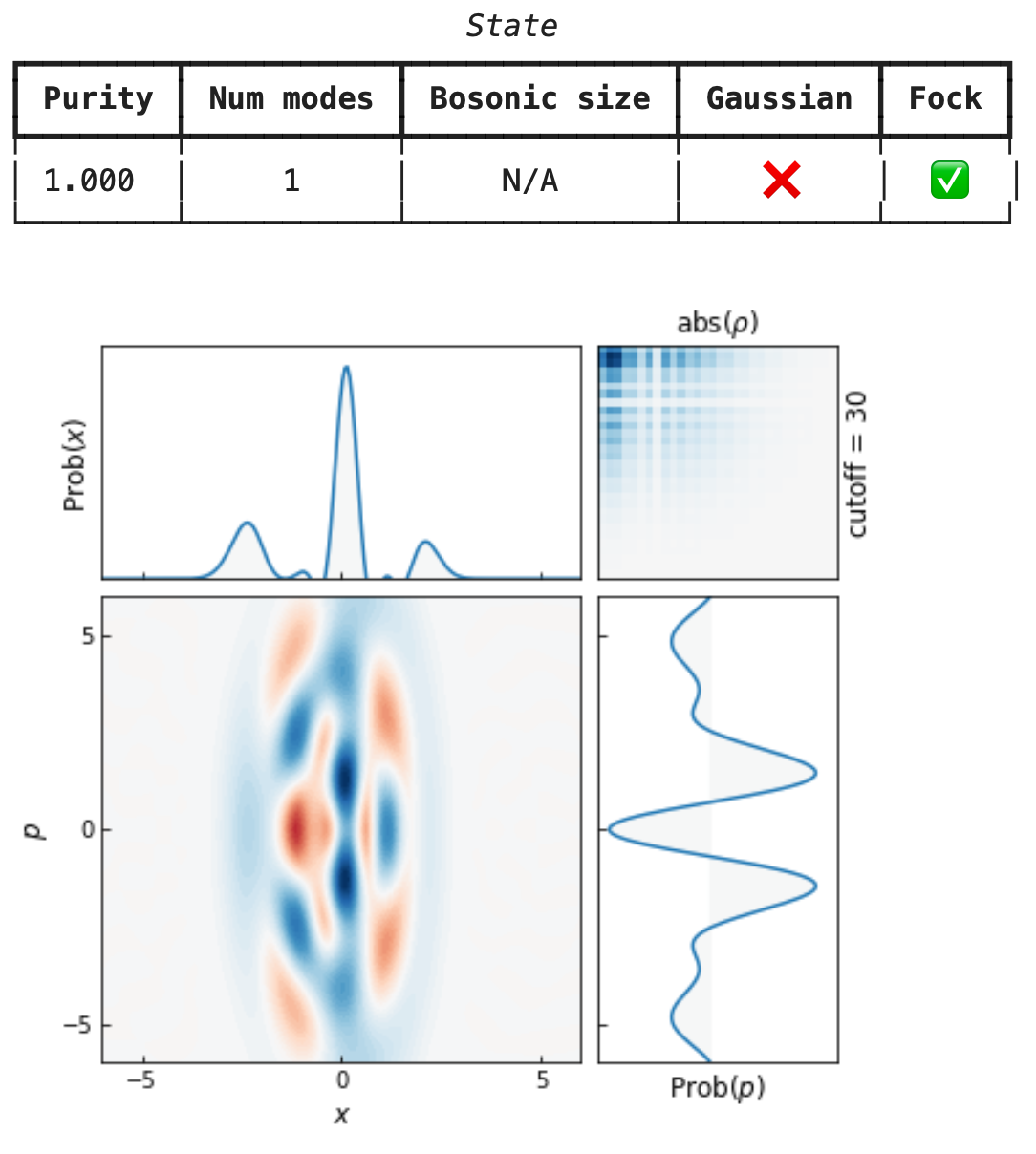
States can be initialized in Fock representation and used as any other state:
my_amplitudes = np.array([0.5, 0.25, -0.5, 0.25, 0.25, 0.5, -0.25] + [0.0]*23)  # notice the buffer
my_state = State(ket=my_amplitudes)
my_state >> Sgate(r=0.5)  # just works
Alternatively,
my_amplitudes = np.array([0.5, 0.25, -0.5, 0.25, 0.25, 0.5, -0.25])  # no buffer
my_state = State(ket=my_amplitudes)
my_state._cutoffs = [42]  # force the cutoff
my_state >> Sgate(r=0.5)  # works too
The physics module
The physics module contains a growing number of functions that we can apply to states directly. These are made out of the functions that operate on the representation of the state:
If the state is in Gaussian representation, then internally the physics functions utilize the physics.gaussian module.
If the state is in Fock representation, then internally the physics functions utilize the physics.fock module.
The math module
The math module is the backbone of Mr Mustard, which consists in the Math interface
Mr Mustard comes with a plug-and-play backends through a math interface. You can use it as a drop-in replacement for tensorflow or numpy and your code will be plug-and-play too!
Here’s an example where the numpy backend is used.
import mrmustard.math as math

math.cos(0.1)  # numpy
In a different session, we can change the backend to tensorflow.
import mrmustard.math as math
math.change_backend("tensorflow")

math.cos(0.1)  # tensorflow
Optimization
The mrmustard.training.Optimizer uses Adam underneath the hood for the optimization of Euclidean parameters, a custom symplectic optimizer for Gaussian gates and states and a unitary/orthogonal optimizer for interferometers.
We can turn any simulation in Mr Mustard into an optimization by marking which parameters we wish to be trainable. Let’s take a simple example: synthesizing a displaced squeezed state.
from mrmustard import math
from mrmustard.lab import Dgate, Ggate, Attenuator, Vacuum, Coherent, DisplacedSqueezed
from mrmustard.physics import fidelity
from mrmustard.training import Optimizer

math.change_backend("tensorflow")

D = Dgate(x = 0.1, y = -0.5, x_trainable=True, y_trainable=True)
L = Attenuator(transmissivity=0.5)

# we write a function that takes no arguments and returns the cost
def cost_fn_eucl():
    state_out = Vacuum(1) >> D >> L
    return 1 - fidelity(state_out, Coherent(0.1, 0.5))

G = Ggate(num_modes=1, symplectic_trainable=True)
def cost_fn_sympl():
    state_out = Vacuum(1) >> G >> D >> L
    return 1 - fidelity(state_out, DisplacedSqueezed(r=0.3, phi=1.1, x=0.4, y=-0.2))

opt = Optimizer(symplectic_lr=0.1, euclidean_lr=0.01)
opt.minimize(cost_fn_eucl, by_optimizing=[D])  # using Adam for D

opt = Optimizer(symplectic_lr=0.1, euclidean_lr=0.01)
opt.minimize(cost_fn_sympl, by_optimizing=[G,D])  # using Adam for D and the symplectic opt for G